
Many engineers haven't had direct exposure to statistics or Data Science. Yet, when building data pipelines or translating Data Scientist prototypes into robust, maintainable code, engineering complexities often arise. For Data/ML engineers and new Data Scientists, I've put together this series of posts.
I'll explain core Data Science approaches in simple terms, building from basic concepts to more complex ones.
The whole series:
- Data Science. Probability
- Data Science. Bayes theorem
- Data Science. Probability Distributions
- Data Science. Measures
- Data Science. Correlation
- Data Science. The Central Limit Theorem and Sampling
- Data Science. Demystifying Hypothesis Testing
- Data Science. Data types
- Data Science. Descriptive and Inferential Statistics
- Data Science. Exploratory Data Analysis
Probability distributions are the hidden force behind so much of what we experience, from how Google predicts traffic to how your favorite app picks the perfect ad to show you. But if you're anything like me, reading about probability distributions often feels like wading through molasses. In this blog post, we're going to break it down — no math degree required.
PDF and CDF
Probability Density Function (PDF)
Let's start with the basics: the probability density function, or PDF. If you've ever wondered, "How likely is it that my favorite TV show will be canceled?" or "What are the odds of landing on heads 5 times in a row?" — you're thinking like a PDF.
Imagine an experiment where each outcome has a different probability. Say you roll a fair die with six sides. Here, each side has an equal 1/6 probability of coming up, but what if your die is lopsided? Let's say it's a homemade, wonky four-sided die with uneven probabilities:
- 1 comes up 10% of the time,
- 2 comes up 20% of the time,
- 3 comes up 30% of the time, and
- 4 comes up 40% of the time.
To make sense of these odds, we can create a function: f(x) = x / 10, where x is the outcome (1, 2, 3, or 4). This function is our PDF — a way to express the chances for each result, based on our rule. When we're dealing with discrete values like these, the PDF is also called a probability mass function (PMF).
Cumulative Distribution Function (CDF)
If the PDF is like picking an individual item from a shelf, the cumulative distribution function (CDF) is like filling up your shopping cart. The CDF answers, "What are the odds of getting any number up to and including this one?" It's cumulative, as the name implies — so, in our four-sided die example, the CDF at 3 would be the total probability of rolling a 1, 2, or 3.
To put it another way, the CDF represents the cumulative probability of values up to a given point. For continuous distributions, it's the integral of the PDF — essentially a sum of probabilities over a range.
Continuous Distributions
Now, what if we want to model situations that aren't just about specific numbers but about ranges? For example, imagine you're trying to predict temperatures, weights, or stock prices. Continuous distributions handle these beautifully, as they model variables that can take on any value within a range, not just whole numbers.
Uniform Distribution
A uniform distribution is where every outcome within a specific range is equally likely; each variable has the same probability. Think about drawing a card from a shuffled deck — each suit or rank has an equal probability. Or consider a coin toss — heads and tails both have a 50% chance.
from scipy.stats import uniform
import matplotlib.pyplot as plt
import numpy as np


def uniform() -> None:
    fig, ax = plt.subplots(1, 1, figsize=(15,15))
    # calculate a few first moments
    mean, var, skew, kurt = uniform.stats(moments='mvsk')
    # display the probability density function (`pdf`)
    x = np.linspace(uniform.ppf(0.01), uniform.ppf(0.99), 100)
    ax.plot(x, uniform.pdf(x),
        'r-', lw=5, alpha=0.6, label='uniform pdf')
    ax.plot(x, uniform.cdf(x),
        'b-', lw=5, alpha=0.6, label='uniform cdf')
    # Check accuracy of `cdf` and `ppf`
    vals = uniform.ppf([0.001, 0.5, 0.999])
    np.allclose([0.001, 0.5, 0.999], uniform.cdf(vals))

    # generate random numbers
    r = uniform.rvs(size=1000)
    # and compare the histogram
    ax.hist(r, normed=True, histtype='stepfilled', alpha=0.2)
    ax.legend(loc='best', frameon=False)
    plt.show()

uniform()
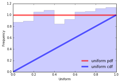
Formally, this is the distribution of a random variable that can take any value within the interval (a, b), and the probability of being in any segment inside (a, b) is proportional to the length of the segment. Values outside the interval have zero probability.
A continuous random variable x has a uniform distribution if its probability density function is:
$$ f(x) = \dfrac{1}{b-a} $$
Normal Distribution
from scipy.stats import norm
import matplotlib.pyplot as plt
import numpy as np


def normal() -> None:
    fig, ax = plt.subplots(1, 1)
    # calculate a few first moments
    mean, var, skew, kurt = norm.stats(moments='mvsk')
    # display the probability density function (`pdf`)
    x = np.linspace(norm.ppf(0.01),  norm.ppf(0.99), 100)
    ax.plot(x, norm.pdf(x),
        'r-', lw=5, alpha=0.6, label='norm pdf')
    ax.plot(x, norm.cdf(x),
        'b-', lw=5, alpha=0.6, label='norm cdf')
    # check accuracy of `cdf` and `ppf`
    vals = norm.ppf([0.001, 0.5, 0.999])
    np.allclose([0.001, 0.5, 0.999], norm.cdf(vals))

    # generate random numbers:
    r = norm.rvs(size=1000)
    # and compare the histogram
    ax.hist(r, normed=True, histtype='stepfilled', alpha=0.2)
    ax.legend(loc='best', frameon=False)
    plt.show()

normal()
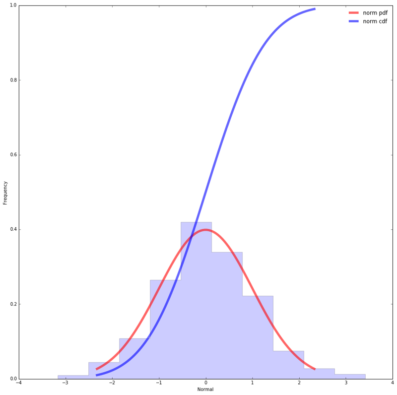
At the heart of statistics lies the normal distribution, often known as the bell-shaped curve. It is a two-parameter family of curves representing plots of probability density functions:
$$ f(x) = \frac{1}{\sigma \sqrt{2\pi}} \exp\left(−\frac{(x−\mu)^2}{2\sigma^2}\right) $$
It looks a little scary, but we'll get it all figured out soon enough. The normal distribution density function has two mathematical constants:
π— the ratio of the circumference of a circle to its diameter, approximately3.142;e— the base of the natural logarithm, approximately2.718.
And two parameters that set the shape of a particular curve:
µis the mean or expectation, showing that data near the mean are more frequent than data far from it.- $#σ^2#$ — variance, will also be discussed in future posts.
And, of course, the variable x itself, for which the function value is calculated, i.e., the probability density.
The constants, of course, don't change, but parameters give the final shape to a particular normal distribution.
So, the specific form of the normal distribution depends on 2 parameters: the expectation (µ) and variance ($#σ^2#$). The parameter µ (expectation) determines the distribution center, which corresponds to the maximum height of the graph. The variance $#σ^2#$ characterizes the range of variation, that is, the "spread" of the data.
When calculating standard deviation, we find that:
- about 68% of values are within 1 standard deviation of the mean,
- about 95% are within 2 standard deviations,
- about 99.7% are within 3 standard deviations.
Why is this distribution so popular?
The importance of normal distributions is primarily due to the fact that the distributions of many natural phenomena are roughly normally distributed. One of the first applications of normal distributions was analyzing measurement errors in astronomical observations, errors caused by imperfect instruments and observers. In the 17th century, Galileo noted that these errors were symmetrical and that small errors occurred more frequently than large ones. This led to various error distribution models, but it was only in the early 19th century that it was discovered that these errors followed a normal distribution.
Independently, mathematicians Adrien-Marie Legendre and Carl Friedrich Gauss in the early 1800s formalized the normal distribution's shape in a formula, showing that errors align with this distribution. Today, it's nearly impossible to imagine fields like statistics, economics, biology, or engineering without it. The beauty of the normal distribution lies in its versatility — many processes, from human height to stock returns, show this pattern, especially as sample sizes grow.
Discrete Distributions
Now, let's zoom in on discrete distributions. These are distributions where possible outcomes are countable, like flipping a coin, rolling a die, or even your work inbox at 9 am — every event has distinct, countable occurrences. The key here is that while continuous distributions spread probability smoothly over a range, discrete distributions assign probabilities to specific values or outcomes.
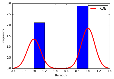
Bernoulli Distribution (and Binomial)
The Bernoulli distribution represents the simplest kind of random experiment: a single trial that has two possible outcomes, usually labeled as "success" and "failure". Imagine a single coin flip, where getting heads might be considered a success and tails a failure. In a Bernoulli distribution, the probability of success (p) remains constant.
Now, let's get a little more interesting. When we repeat that Bernoulli experiment a bunch of times — say, flipping a coin ten times and counting how many times it lands heads — that's when we move to the Binomial distribution. Essentially, the Binomial distribution gives us the probability of observing exactly k successes in n trials, each with a success probability of p.
from scipy.stats import bernoulli
import seaborn as sb


def bernoulli_dist(): -> None:
    data_bern = bernoulli.rvs(size=1000,p=0.6)
    ax = sb.distplot(
        data_bern,
        kde=True,
        color='b',
        hist_kws={'alpha':1},
        kde_kws={'color': 'r', 'lw': 3, 'label': 'KDE'})
    ax.set(xlabel='Bernouli', ylabel='Frequency')

bernoulli_dist()
But not all phenomena are measured on a quantitative scale like 1, 2, 3, ... 100500. Many phenomena have a limited set of possible outcomes instead of an infinite range. For example:
- A person's gender can be classified as male or female.
- A shooter can either hit or miss the target.
- A voter may vote either "for" or "against" a measure.
In these cases, we have a binary outcome, where one result represents a positive outcome, or "success". Such phenomena may also involve randomness, which makes them perfect candidates for probabilistic and statistical modeling.
Experiments with binary outcome data are modeled using the Bernoulli scheme, named after the Swiss mathematician Jacob Bernoulli. He discovered that with enough trials, the ratio of positive outcomes (successes) to the total number of trials converges to the probability of a positive outcome occurring. This leads to the binomial probability formula:
$$ f(x) = \dbinom{n}{x} p^x (1-p)^{n-x} $$
Where:
nrepresents the number of experiments in the series,xis a random variable representing the number of occurrences of the event,pis the probability of success in a single trial,- and
q = 1 - pis the probability that the event does not occur in a trial.
This setup is especially useful in scenarios where events are independent and each trial has the same success probability — like predicting the likelihood of a certain number of heads in a series of coin flips or the chance that a specific number of customers make a purchase out of a large group visiting an online store.
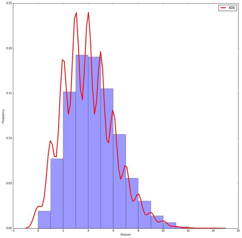
Poisson Distribution
The Poisson distribution comes in handy when you're looking at the frequency of events within a specific interval. Let's say we're counting the number of emails you get each hour (and, wow, do we know the pain). This distribution is perfect for that situation because it gives us the probability of a certain number of events happening in a fixed period, given that the events happen at a constant average rate.
Formally, the Poisson distribution is often described as a limiting case of the Binomial distribution. When the number of trials gets very large (n → ∞), and the probability of success becomes very small (p → 0), but their product (n*p) stays constant, we get a Poisson distribution.
from scipy.stats import poisson
import seaborn as sb
import numpy as np
import matplotlib.pyplot as plt


def poisson_dist(): -> None
    plt.figure(figsize=(15,15))
    data_binom = poisson.rvs(mu=4, size=10000)

    ax = sb.distplot(data_binom, kde=True, color='b',
                    bins=np.arange(data_binom.min(), data_binom.max() + 1),
                    kde_kws={'color': 'r', 'lw': 3, 'label': 'KDE'})
    ax.set(xlabel='Poisson', ylabel='Frequency')

poisson_dist()
The Poisson distribution is obtained as a limiting case of the Bernoulli distribution, if we push p to zero and n to infinity, but so that their product remains constant: n*p = a. Formally, such a transition leads to the formula
$$ f(x) = \frac{{e^{ - \lambda } \lambda ^x }}{{x!}} $$
Where:
xis the number of occurrences,λrepresents the average event rate within a given interval.
Imagine you're in charge of a customer support center and want to predict the number of calls during a lunch break. The Poisson distribution is ideal because it's all about counting events over time. Any random event that follows a stable average rate, like traffic on a website or bus arrivals at a station, can be modeled with Poisson. However, keep in mind it works best when events are independent, and occurrences are relatively rare within each interval.
Conclusion
There are many theoretical distributions—Normal, Poisson, Student, Fisher, Binomial, and others—each designed for analyzing different types of data with specific characteristics. In practice, these distributions are often used as templates to analyze real-world data of similar types. Essentially, they provide a structure that analysts can apply to real data, allowing them to calculate characteristics of interest based on the distribution's properties.
More precisely, theoretical distributions are probabilistic-statistical models used to interpret empirical data. The process involves collecting data and comparing it to known theoretical distributions. If there are strong similarities, the properties of the theoretical model are assumed to hold for the data, allowing analysts to draw conclusions. This is the foundation for classical methods such as hypothesis testing, which includes calculating confidence intervals, comparing mean values, and testing parameter significance.
However, if the data doesn't fit any known theoretical distribution (which, in practice, happens more often than we admit), using a forced template can lead to misleading results. It's like searching for your keys where the light is best rather than where you actually dropped them. To address this, there are alternative approaches, such as non-parametric statistics, that provide more flexibility when data doesn't follow a standard pattern.
Additional materials
- MIT Introduction to Probability
- Intro Probability Theory
- Practical Statistics for Data Scientists
- Naked Statistics: Stripping the Dread from the Data