BigQuery Explained: What Really Happens When You Hit “Run”
⚠️ Warning: This isn't a "what is BigQuery?" explainer. It's a deep, systems-level breakdown aimed at engineers who want to know how the machine actually works.
BigQuery is an "infinite cluster" that feels like magic. You write some SQL, hit "Run", and seconds (or sometimes minutes) later, the answer comes back — even if the data is measured in petabytes.
No servers around. No cluster in the traditional sense. No JVM babysitting. No Spark version drama. You don't size your storage. You don't manage compute. You just ask a question — and for a few seconds, Google's infrastructure wakes up, fans out across thousands of CPUs, gets the job done, and then vanishes after returning the results.
In this blog post, I'll break down what actually happens under the hood. We're not doing this for trivia points. Understanding the rough shape of BigQuery's internals helps you reason about why certain queries are slow or expensive, why clustering and partitioning matter so much, and what knobs you actually still have in a "serverless" system. We'll look at the design decisions that define how BigQuery works, and why it behaves the way it does. Ready?

The Source Story
Before we dive into the moving parts, it's helpful to understand where BigQuery came from — and why it looks so different from traditional data warehouses.
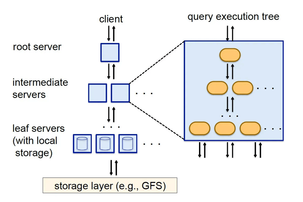
In 2010, Google published the Dremel paper, which described how internal analysts could query trillions of rows in seconds.
This might sound routine today, but remember: this was still peak Hadoop era. The ecosystem was a mess of Hive-on-MapReduce jobs, cron-driven ETLs, and people proudly hoarding CSVs on HDFS. Most "analytics" meant waiting for a job to finish — not running interactive SQL.
Dremel changed that.
Instead of relying on linear scans or brittle indexes, Dremel was designed for interactive querying at massive scale. Its core design decisions shaped what would later become BigQuery:
- Native nested data: Dremel treated
STRUCTs andARRAYs as first-class citizens. It could query deeply nested, semi-structured data (like Protocol Buffers or JSON-like structures) without forcing you to flatten or denormalize everything. That was huge. It meant you could keep your rich data model without blowing up your query complexity. - Columnar storage: Again, obvious now — but not in 2010. Storing data column-by-column allowed tight compression, faster reads, and only scanning what you need. Remember, row-based formats like Avro were still common. ORC and Parquet hadn't hit full adoption yet.
- Tree-based execution: Instead of shuffling everything around like in MapReduce, Dremel built a multi-level aggregation tree. Each node processed partial results and passed them up optimizing for latency instead of throughput.
That heritage explains why BigQuery likes wide, read‑heavy tables. It explains why nested data isn't a second‑class citizen and why the engine is optimized to skip work instead of muscling through it.
The idea is to write and store data in ways that make skipping easy. It's about doing as little work as possible.
You can sort of think of BigQuery as Dremel-as-a-service, though that's a bit of an oversimplification. The Dremel model still powers the query engine, but modern BigQuery has evolved far beyond that into something closer to a serverless, distributed operating system for SQL.
So how does that system actually work?
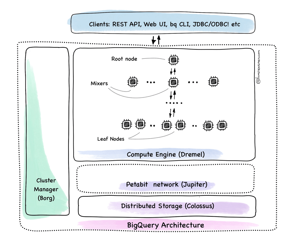
Architecture
To understand BigQuery, you have to stop thinking like you're working with a traditional database. There's no Postgres instance where you know exactly where your index lives and what the page size is. This is something else entirely.
BigQuery is designed more like a distributed OS — a layered system that handles storage, scheduling, execution, metadata, and coordination — and lets you interact with it through SQL.
We'll break it down not by product feature, but by how data actually flows when you run a query. We'll start at the very bottom (storage) and work our way up to coordination, execution, and result delivery.
Storage: Capacitor + Colossus
All BigQuery data sits on Colossus — Google's internal storage system. And no, it's not just another HDFS clone or S3.
HDFS vs. Colossus
HDFS is built around a centralized model: a single NameNode holds all the metadata, and DataNodes store the actual data. It works fine for small to mid-sized clusters, but once you scale to thousands of nodes, it starts to crack. Metadata becomes a bottleneck, and adding more machines doesn't linearly increase throughput.
Colossus does things differently. It splits metadata and data storage completely. Metadata lives in high-performance NoSQL database, Bigtable, while actual data blocks are spread across independent storage nodes — built to scale and survive massive failures, even full data centers going offline. No single point of failure. No metadata choke point.
Colossus doesn't give you filenames, paths, or a tree. It's not a file system in the traditional sense. You write a blob, you get a handle back. That handle is opaque — you can't peek inside or ask where your data went. And you're not supposed to.
But the system knows. Look at the diagram.
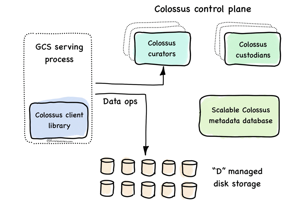
The Colossus client library, embedded in the GCS (Google Cloud Storage) serving process, talks to the metadata layer — backed by Bigtable (aka Scalable Colossus metadata database in the diagram above) — which knows exactly where each blob lives and how it's replicated. Data goes directly to and from the managed disks, bypassing any central data path.
Behind the scenes, the control plane — curators and custodians — quietly keeps the system alive: healing broken replicas, optimizing layout, rebalancing load. The client never sees them.
That's what makes the opaque interface work: Colossus can move your data, rewrite it, or repair it without coordination or downtime. Compare that to HDFS, where clients have to talk to the master and track block locations themselves. Colossus is smarter. And quieter.
Like S3?
And while it might look similar to S3 — no file paths, no directories, opaque object handles — it's not the same beast. S3 is a general-purpose object store exposed over HTTP, built to serve a wide range of workloads over the open internet. Colossus, on the other hand, is tightly wired into Google's internal stack. It's RPC-based, not HTTP — which means lower latency, less overhead, and tighter control over semantics.
But it goes deeper than the protocol.
The key difference is how deeply Colossus is wired into Google's internal stack. Its metadata is backed by Bigtable, its storage nodes run as Borg-scheduled processes, and its control plane continuously monitors disk health, repairs replicas, and rebalances data — all automatically and invisibly to clients.
In other words, Colossus isn't a separate service you "call". It's part of the machine. When BigQuery writes or reads data, it's not making a network request to some external thing — it's interacting with an internal system that already knows what job is running, where it's scheduled, and how to move data efficiently. You don't "upload a file" — you stream data straight into the machine, and everything downstream knows what to do with it.
Capacitor
BigQuery doesn't use Parquet or ORC under the hood. It has its own columnar format called Capacitor — purpose-built to run on top of Colossus.
Capacitor is also columnar, but not in the same way Parquet is. Capacitor's design is a lot more aggressive. Every column is broken into independently addressable chunks, and each chunk carries its own metadata — zone maps (min/max), encoding info, null counts, row count, the works. The chunks can be skipped individually during scan, which matters a lot when you're dealing with petabytes.
Compression is built-in and automatic. It picks from multiple encodings (dictionary, RLE, delta, bit-packing — things we've talked before), and it adapts — no knobs to tweak, no configs to mess with. Typical compression ranges from 5x to 15x depending on data shape. You as a user don't have to do anything to get that — it just happens.
The layout is truly column-first, including nested data. Capacitor stores each nested field as its own stream, with structural metadata mapping parent-child boundaries. They don't get flattened. So if you have a column like:
STRUCT<user_id STRING, events ARRAY<STRUCT<type STRING, ts TIMESTAMP>>>
Capacitor stores events.type separately from events.ts, separately from user_id. That means you can scan events.type without reading ts, or even touching user_id. No shredding, no exploding, no backfilling nulls into fake rows like some other warehouses do.
This layout is strictly column-first, even for complex types. That's what enables efficient predicate pushdown and selective scans.
This design illustrates why partitioning and clustering matter. Clustering and partitioning let the planner rule out entire chunks of data at the scan phase: full partitions, full column blocks, full zone ranges. You're not speeding up the engine — you're giving it a reason not to run at all.
Physical execution: slots, tree, stages, shuffle
This is a premium deep-dive
You just read the free excerpt. The full analysis continues on Substack.
Read full article → Or subscribe to get all premium posts